PDF Summary:The Art of Uncertainty, by David Spiegelhalter

Most people don’t handle uncertainty well—we rely on gut feelings and vague language like “probably” or “likely” that mean different things to different people. In The Art of Uncertainty, statistician David Spiegelhalter reveals why our intuitions about uncertainty mislead us and offers a better approach: probabilistic thinking. His central insight challenges conventional wisdom: He says that probability isn’t an objective feature of reality, but a tool for quantifying personal uncertainty.

If you master Spiegelhalter’s method for dealing with uncertainty, you’ll make better predictions, communicate risks clearly, and avoid both overconfidence and excessive caution. You’ll learn why most “coincidences” are statistically inevitable, how to update beliefs when facing new evidence, and why intellectual humility beats false certainty. Along the way, you’ll discover why debates about probability determine what questions science can answer, you’ll learn how intuition regularly misleads you when it comes to randomness and risk, and you’ll see why forecasts can sometimes be right for the wrong reasons.

(continued)...

Why Numbers Beat Words for Expressing Uncertainty

Spiegelhalter argues that numbers provide precision that words can’t. People express uncertainty using words like “likely,” “possible,” “probable,” or “rare,” but these mean different things to different people. Drug regulators call side effects that occur between 1% and 10% of the time “common,” but patients assume a “common” side effect is much more prevalent. However, when Silver assigned Trump a 28.6% probability of winning the 2016 election, this communicated something specific: In 100 similar situations, we’d expect that outcome roughly 29 times.

Spiegelhalter points out that expressing uncertainty numerically enables accountability over time. If Silver had said Trump’s victory was “unlikely” or “possible,” we couldn’t evaluate whether his judgment was well-calibrated. But because he’s provided numbers for hundreds of races over multiple election cycles, we can check: Do candidates he gives 70% odds win roughly 70% of the time? Do those he gives 30% odds win roughly 30% of the time? This reveals whether he’s overconfident (claiming more certainty than warranted), underconfident (hedging too much), or well-calibrated (his numbers match reality). With words like “likely” or “probably,” no such evaluation is possible because everyone interprets the terms differently.

The Limits of Calibration: What “Well-Calibrated” Really Means

With over thousands of predictions made since 2008, Nate Silver’s forecasts have proven well-calibrated: Events he said had a 70% chance of occurring happened 71% of the time, and events with a 5% chance happened 4% of the time. This is how we typically evaluate probabilistic forecasts: not by whether any single prediction was “right” or “wrong,” but by whether stated probabilities match outcome frequencies across many predictions. But some experts argue calibration isn’t a useful measure of forecast quality because it measures whether your numbers match outcomes, but it doesn’t capture whether your reasoning was sound.

Researchers have shown that given enough time and predictions, anyone can achieve good calibration—even people who know nothing about what they’re predicting—by adjusting how they group their forecasts. This means that a forecaster can be right (and well-calibrated) for the wrong reasons, making faulty assumptions that just happen to produce accurate probabilities. Consider the kinds of assumptions Silver’s model makes about an election: that polling errors in Pennsylvania will correlate with errors in Wisconsin and Michigan because they have similar demographics; that the 2.5% general bias in past elections will apply to future ones; or that economic indicators like the GDP will influence voters in predictable ways.

Any of these assumptions could be wrong, but a forecaster could still appear well-calibrated if their errors happen to cancel each other out, or if they’re lucky with the specific elections they forecast. Calibrating for US presidential elections faces a particularly harsh constraint: Determining whether one model is really better than another would require decades or even centuries of data, since there’s only one presidential election every four years. We can see that Silver’s modeling choices have worked well, but we can’t prove they’re optimal instead of lucky, due to the small sample of elections we’ve observed.

What Probability Actually Means

Now that we understand probability as a numerical tool for quantifying uncertainty, a deeper question remains: What do these numbers actually represent? Do they describe something real about the world, or are they just useful fictions we construct? Spiegelhalter takes a philosophical stance that distinguishes his approach from standard statistics textbooks, but understanding his position requires examining what probability could mean according to different interpretations that have developed over time.

How Different Philosophical Approaches Lead to Different Understandings

The debate over what probability “really means” parallels debates in quantum physics about whether mathematics describes something real or is just a useful tool. As Adam Becker explains in What Is Real?, physicists agree on quantum theory’s math but disagree as to what it represents: Do particles actually exist in multiple states at once, and instantaneously affect each other across long distances, or is that just how the math works?

Similarly, statisticians agree on how to calculate probabilities while disagreeing about what the numbers say about the world. For example, when we say there's a 60% chance of rain tomorrow, does that describe an objective feature we could measure by observing many similar days, or does it express our personal degree of certainty given current weather data? This question matters because it determines what questions probability can legitimately answer, a practical issue we’ll see emerge as we examine each view.

The Classical View: Probability Comes From Symmetry

Spiegelhalter explains that the classical view defines probability through physical symmetry: A coin toss has a 50% probability for heads because two equally likely outcomes exist and nothing favors one over the other. This view works for dice, coins, and cards, but it struggles elsewhere. What’s the probability of rain tomorrow? There’s no symmetry to appeal to, and calling outcomes “equally likely” presumes we know the probabilities.

(Shortform note: The classical view treats randomness as physical indifference—a die has no preference for any outcome because of its symmetrical structure. This makes probability objective—the chance of 1/6 for each face exists independent of any observer—but extremely limited as a tool: You can only apply it to systems with clear physical symmetry. This is why the classical view can’t meaningfully discuss “the probability it will rain tomorrow.” There’s no physical symmetry that makes rain and sunshine equally probable.)

The Frequentist View: Probability Is What Happens in Infinite Repetitions

The frequentist view, dominant in science, defines probability as the long-run proportion that would emerge if you could repeat the same situation indefinitely. Spiegelhalter explains that if we could flip a coin over and over without limit, the proportion landing on heads would approach 50%. This appeals to scientists because it’s based on observable frequencies. If a drug works for 70 out of 100 patients, we can estimate future probability from this frequency. But Spiegelhalter argues that this view faces serious limitations.

First, how do we apply this interpretation of probability to one-time events? An election will happen once: We can’t re-run it infinitely to see what proportion of times each candidate wins. The frequentist definition seems to suggest these one-time events don’t have meaningful probabilities at all. Second, even when repetition seems possible, deciding what counts as “the same situation” requires judgment. For instance, is every patient similar enough to those in clinical trials? Two patients are never identical—they differ in age, genetics, lifestyle, and countless other factors. Determining which differences matter and which can be ignored involves subjective decisions about what situations are “similar enough” to group together.

(Shortform note: The frequentist view extends probability beyond symmetrical systems by defining it through observed patterns. Unlike the classical view where probability reflects a coin’s structure, the frequentist view says 50% probability represents the pattern that emerges from repeated observation. This is the view that can model weather: If you could observe thousands of similar days, rain would occur on a certain proportion of them. Here, randomness is treated as real—nature is genuinely indeterministic—and probability is objective (there’s a definite long-run frequency). But this only works for repeatable processes, which is why frequentists struggle with one-time events like elections.)

Spiegelhalter’s Subjective View: Probability Quantifies Personal Uncertainty

Spiegelhalter adopts a fundamentally different position: Probability represents a personal degree of belief based on an individual’s current knowledge and judgment, not objective features of the external world. When you say there’s a 60% chance of rain tomorrow, you’re not claiming to have measured some objective property of the weather system. You’re expressing your personal degree of certainty given what you know about weather patterns, forecast models, and atmospheric conditions. Someone with different information—perhaps a professional meteorologist with access to more detailed data—might reasonably assess the probability as 50% or 70%. Neither of you is objectively “right” or “wrong.”

The subjective view doesn’t deny that some probability assessments are better than others. It just recognizes that probability is a tool we use to organize our thinking about uncertainty, not a property of the world we can passively observe—probabilities represent judgments, not objective measurements made with instruments like thermometers or scales. Nevertheless, probabilities can still be evaluated for quality; they must connect to reality and can be tested against outcomes. If you consistently claim 60% confidence for events that occur only 30% of the time, your probability assessments are poorly calibrated.

This subjective interpretation has three practical implications:

First, probability applies meaningfully to one-time events. You can discuss the probability that Lee Harvey Oswald acted alone in assassinating President John F. Kennedy, or that Shakespeare wrote all the plays attributed to him, or that a particular company’s new product will succeed, because these probabilities measure your degree of certainty, not a repeatable likelihood.

Second, expert disagreement about probabilities doesn’t mean someone must be objectively wrong: Conflicting assessments can be legitimate quantifications of uncertainty from different perspectives.

Third, this view makes clear that all probability assessments involve judgment and interpretation, requiring honesty about the limits of our knowledge rather than false claims to objectivity.

(Shortform note: The subjective view treats “randomness” as a reflection of our ignorance rather than true indeterminacy. A coin flip’s outcome is determined by velocity, air resistance, and other physical factors, but we call it “random” because we can’t measure these precisely. What matters is that we’re uncertain, regardless of whether that’s because reality is probabilistic or because it’s deterministic but we have incomplete knowledge. This is why most statisticians sidestep the philosophical debate entirely: They treat probabilities as quantifying uncertainty given available information, focus on whether their models work rather than what they “really mean,” and stay open to updating predictions as new evidence emerges.)

Learning From Evidence: Bayesian Updating

If probability represents personal belief rather than objective fact, a question follows: How should our beliefs change when we encounter new evidence? This is where “Bayesian updating” enters Spiegelhalter’s framework. Named for 18th-century mathematician Thomas Bayes, Bayesian updating provides the mathematically correct way to revise subjective probabilities in light of new evidence. Bayes solved a fundamental problem: Given what you believed before (your prior probability) and given a new piece of evidence, what should you believe now (your posterior probability)? Bayes’ theorem shows how to combine your prior belief with new information to arrive at a logically consistent updated belief.

Bayes’ logic is straightforward: Your updated belief should reflect what you thought before and what the new evidence suggests. If you initially thought something was very unlikely but you then find a hint of evidence supporting it, you should increase your belief that it’s true, but only somewhat. Your prior belief matters because it captures everything you knew before new evidence arrived.

How Quickly Should You Update Your Beliefs?

Updating your beliefs with new evidence is important—but so is resisting hasty revisions based on noisy data. A study of blue whale migration illustrates this principle. Scientists long assumed migrating blue whales tracked phytoplankton blooms in real time, adjusting their routes each year to follow where the phytoplankton—and thus the krill the whales feed on—were most abundant. To test this, researchers tracked 60 whales over a decade and compared their paths to two things: where that year’s blooms actually occurred, and the long-term average pattern of where blooms typically occur over many years.

The surprising finding: The whales’ paths matched the 10-year average bloom pattern far better than any individual year’s actual bloom locations. The whales followed historical patterns rather than chasing current conditions, which makes sense because any single year’s bloom might appear in an unusual location due to temporary weather patterns. By relying on long-term memory of where food is usually abundant, whales avoid being misled by year-to-year fluctuations. The scientists demonstrated the same principle, collecting a decade of data before revising their hypothesis about how blue whales choose their migration paths.

Spiegelhalter illustrates how Bayes’ theorem can play out in the real world with an example of a facial recognition system. Imagine that such a system scans a crowd of 10,000 people containing 10 suspects on a watchlist. The system correctly identifies 70% of the suspects and produces false alerts for only 1 in 1,000 innocent people (a 0.1% false alarm rate).

Now suppose the system flags someone. Should security detain them? Your intuition might be to focus on the system’s accuracy: a 70% correct identification rate with only 0.1% false alarms sounds reliable. But Bayesian reasoning reveals a different picture: The system would correctly identify 7 of the 10 suspects (70% of 10) and falsely flag 10 innocent people (0.1% of 9,990). In total, 17 people get flagged: 7 actual suspects and 10 innocent bystanders. Thus, if a person is flagged, there’s only a 7-in-17 chance—roughly 41%—that they’re on the watchlist. Despite the system’s impressive accuracy rates, the people it identifies are more likely to be innocent than guilty. Why does this happen?

The base rate—the rarity of what you’re looking for—matters enormously. Suspects make up only 0.1% of the crowd (10 out of 10,000). When you’re searching for something extremely rare, most of your alerts will be false alarms because there are many more opportunities for false positives than there are for true identifications. This is Bayesian reasoning in action: The prior probability (before being flagged) that any person in the crowd is a suspect was 0.1%. The new evidence (being flagged) updates this probability, since the system is more likely to flag suspects than innocent people. Bayes’ theorem quantifies how much to update: from a 0.1% to a 41% chance that someone is a suspect on a watchlist.

This increase from 0.1% to 41% seems substantial, but it’s less than most people intuitively expect when they hear that someone has been flagged by a highly accurate facial recognition system—many would assume the probability jumps to 80% or 90%. But, because the base rate was so low, it keeps the system’s level of certainty modest. This systematic approach to updating beliefs provides the foundation for thinking clearly about uncertainty.

The Cognitive Bias That Skews Bayesian Thinking

Base rate neglect—the tendency to ignore how common something is in the population—is a persistent cognitive bias that affects us even when we consciously know the base rate. An online comic illustrates this with the claim that “right-handed people make 90% of all base rate errors.” We might facetiously assume this means that right-handed people are worse at avoiding base rate neglect, but it really means that the proportion of people making base rate errors reflects the fact that 90% of people are right-handed.

In this case, the base rate neglect is presented in a way that’s obvious (and to comical effect), but we make this error consistently in many situations. Research suggests two main reasons why:

• We give too much weight to information that seems directly relevant while dismissing base rate statistics as less important.

• We focus on how well characteristics match our stereotype of a group rather than considering how common that group really is.

In the comic’s example, the percentage of errors made by right-handed people is framed as important information, while the proportion of people who are right-handed might feel like trivia we can safely ignore. We might even have a stereotypical idea that left-handed people somehow think differently, leading us to expect they’d avoid this error. This same bias explains why Spiegelhalter’s facial recognition example feels so counterintuitive—the 70% accuracy rate and 0.1% false alarm rate seem highly relevant and specific, which makes it easy to overlook the base rate statistic that says suspects are vanishingly rare in the crowd.

How to Navigate Uncertainty in Practice

Having the right mathematical tools to quantify our uncertainty and update our predictions isn’t enough—we also need strategies to apply these tools in messy real-world situations where our models might be wrong and our knowledge is incomplete. In this section, we’ll explore Spiegelhalter’s practical principles for handling uncertainty when it matters most: distinguishing causation from correlation, communicating uncertainty honestly, understanding extreme events, and maintaining intellectual humility throughout.

1. Distinguish Correlation from Causation

One of the most common errors in reasoning about uncertainty is assuming that because two things occur together, one must cause the other. Spiegelhalter writes that establishing genuine causation requires far stronger evidence than mere correlation. Yet people, including researchers, routinely assume causal connections instead of looking for corroborative evidence from multiple sources.

For example, numerous studies show that teenagers who spend more time on social media report higher rates of depression and anxiety. Many have concluded that social media use causes mental health problems, driving calls for age restrictions and platform regulations. But does social media actually cause depression, or do depressed teens simply spend more time online? Or could a third factor—like having fewer in-person friendships—be causing both increased social media use and increased depression?

Establishing causation in this case is difficult because we can’t randomly assign teenagers to different levels of social media use for years—it would be unethical and impractical. Spiegelhalter says that randomized controlled trials are the gold standard for establishing causation because random assignment ensures that the groups in a study differ only by chance. Cross-sectional studies (such as looking at many teens at one point in time) can show correlation but can’t prove causation. Longitudinal studies (following the same teens over time) help determine whether social media use precedes depression symptoms, but can’t rule out confounding factors.

Why Randomized Controlled Trials Help Establish Causation

Distinguishing correlation from causation is notoriously difficult. When we simply observe what happens to people who make different choices—whether selecting medical treatments, schools, or business strategies—we can’t tell whether the choice caused the outcomes or whether people who chose differently were already different in ways that affected results. Randomized controlled trials (RCTs) solve this problem: Random assignment ensures that the treatment and control groups are comparable on all factors (ones we can and can’t measure) because chance determines who gets which treatment. This is why RCTs can establish causation even when we don’t fully understand all the factors that might affect the outcome.

That said, RCTs have limitations, particularly in medical and social science research where they’re commonly used. They’re often too small or too short to detect rare or long-term harms. They can be unethical if they’re used when there’s no genuine uncertainty about which treatment is better, infeasible for studying long-term outcomes, or prohibitively expensive. RCTs also study people under tightly controlled conditions, which can limit how well results apply to real-world settings, including in fields like economics or education. For these reasons, observational studies remain valuable: They can examine real-world conditions, study rare outcomes over time, and investigate questions where randomization isn’t possible. The ideal is often to triangulate evidence from RCTs and observational studies to build a complete picture.

2. Admit Your Uncertainty

Prediction always involves uncertainty, but the degree of uncertainty varies depending on what you’re predicting and how far ahead you’re looking. Weather forecasting illustrates how this works. Meteorological models can predict the weather two days ahead quite accurately. Seven days ahead, their accuracy drops but remains useful. Beyond about 10 days, forecasts are much less useful because atmospheric conditions are chaotic, so meteorologists use ensemble forecasting, running multiple simulations with varied conditions. Spiegelhalter explains that you should match your approach to the time horizon and degree of certainty. It’s also crucial to be frank when uncertainty runs too deep to make reliable predictions.

(Shortform note: Beyond a certain threshold of uncertainty, the goal shifts from predicting what will happen to building systems that can handle whatever occurs. For example, when space agencies think about future deep space missions or interstellar travel, they don’t know what tech will exist, what biological effects crews will experience, or what problems will arise. So instead of trying to forecast every scenario, they plan for adaptability. For example, NASA is researching how to train four-person Mars crews to handle emergencies that currently require more than 80 experts by preparing for unpredictability. Similarly, experts planning for extraterrestrial contact are designing flexible protocols that can adapt to radically different scenarios.)

Spiegelhalter argues that it’s crucial to be honest about your degree of certainty in your predictions. Many people assume that expressing uncertainty undermines credibility. Spiegelhalter argues the opposite: Transparency about uncertainty builds trust, while false certainty erodes it. It’s important to use numbers rather than words whenever possible, and to provide absolute risks alongside relative risks. The goal should always be to inform people about possibilities rather than to persuade them to see things your way, and to preempt misunderstandings by anticipating how people might misinterpret information.

Why Headlines About Relative Risk Are Often Deceptive

As Spiegelhalter notes, understanding the difference between absolute and relative risk is crucial for interpreting health claims accurately. Absolute risk is the actual probability of an event occurring. For example, if 16 out of every 100 people in a population develop dementia, the absolute risk is 16%. Relative risk compares the probability between two groups as a ratio. If people who regularly solve crossword puzzles have a 12.8% dementia risk versus 16% in non-solvers, the relative risk is 12.8/16 = 0.80, or a 20% relative risk reduction.

This distinction matters because headlines often exploit relative risk to make findings sound more impressive than they are. If you read that “crossword puzzles reduce dementia risk by 20%,” that dramatic-sounding statement refers to relative risk—a 20% reduction in the baseline rate. But the absolute risk only drops from 16% to 12.8%—a reduction of just 3.2%. Both numbers are mathematically correct, yet create vastly different impressions of benefit.

Transparency about this gap between relative and absolute risk matters a lot, especially for situations as frightening as dementia. Also, the research on crossword puzzles only shows correlation, not causation: Studies haven’t established whether regularly completing crossword puzzles actually prevents dementia or whether people with healthier brains are simply more inclined to do puzzles. The most honest assessment from a neurologist might be that doing a crossword puzzle every day won’t hurt you, but your doctor can’t promise that it will protect you against cognitive decline.

3. Understand Extreme Events Without Overreacting

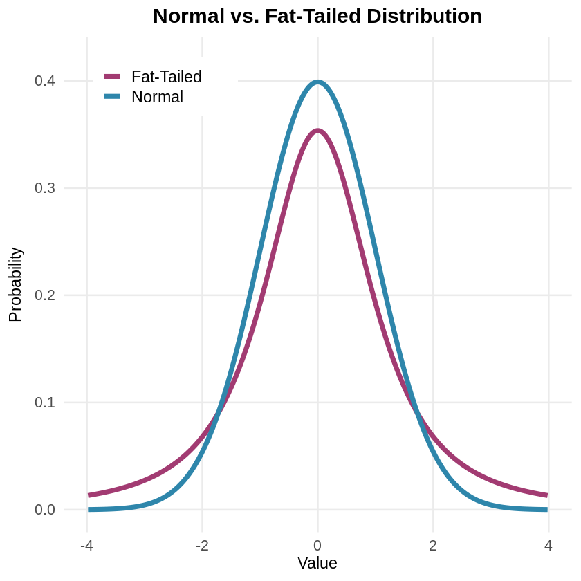
Our intuitions about extreme events mislead us because we expect data to cluster tightly around the average. Normal distributions (visualized with a classic bell curve) describe many phenomena—most values cluster near the average, with fewer and fewer appearing as you move toward the extremes. But financial markets, disasters, and pandemics follow fat-tailed distributions where extremes happen far more frequently. This explains why supposedly “one-in-a-million” events keep happening.

Spiegelhalter explains that understanding this helps us appropriately prepare for catastrophic events, so that we neither ignore the possibility that rare events will happen nor overreact when they occur. For example, after 9/11, the US implemented airport security measures requiring travelers to remove their shoes, limit liquids, and go through full-body scanners. These procedures cause massive delays, cost billions annually, and create stress for millions of travelers. Yet experts agree that TSA screening catches very few actual threats—and that the same resources would save more lives if directed toward other safety measures, like highway improvements.

Understanding Why Extreme Events Happen More Often Than We Expect

The major difference between normal distributions and fat-tailed distributions lies in how quickly probability decreases as you move away from the average. A standard deviation is a statistical measure of how values spread out from the average. In a normal distribution, about 68% of values fall within one standard deviation of the mean, 95% within two standard deviations, and 99.7% within three. Beyond that, probabilities drop off exponentially fast: An event eight standard deviations from the mean has essentially zero probability (0.0000000000000006). Many real-world phenomena (for example, the height of people) follow normal distributions because they result from averaging many small, independent effects.

But Niall Ferguson explains in Doom that disasters follow what statisticians call “power laws” rather than normal distributions. Power laws mean that as disasters get larger, their frequency decreases much more gradually than in a normal distribution. This creates fat-tailed distributions in which extreme events that are eight standard deviations from the norm might occur with a 4% probability. For example, in financial markets, this means a catastrophic crash might happen roughly once every 25 years of trading, rather than essentially never.

Because of power laws, there’s also no “typical” disaster size. In normal distributions, most values cluster tightly around an average. But because power laws spread probability more evenly across different magnitudes, small earthquakes happen frequently, medium ones happen less often, and catastrophically large ones—like magnitude 8.0 earthquakes that release 1,000 times more energy than magnitude 6.0—are rare, but not impossibly so. This pattern also explains why financial crashes, pandemics, and natural disasters consistently surprise us: They happen more frequently than our everyday experience suggests, yet rarely enough that we’re never quite prepared and can easily over- or under-react when they occur.

4. Maintain Intellectual Humility

Finally, we need to exercise intellectual humility, acknowledging that our models are imperfect, our probability assessments are uncertain, and surprises will inevitably occur. Spiegelhalter advises to never assign exactly 0% or 100% probability to anything unless it’s logically impossible or certain. Always leave a small probability, even 1%, that your entire framework might be wrong. If you’re told two bags contain different colored balls and you draw balls to figure out which bag you have, you won’t discover if someone secretly filled both bags identically unless you assigned a small probability to the possibility that “my assumptions are wrong.”

The payoff of humility is adaptability. When you acknowledge uncertainty and stay open to the possibility that your understanding of the situation is wrong, you can update your beliefs quickly when reality diverges from expectations. Spiegelhalter sees humility as the foundation for learning from experience and making better judgments over time in an uncertain world.

(Shortform note: The statistical models we use to understand and predict uncertain outcomes are always imperfect simplifications of a complex reality, which is why statisticians say that “All models are wrong, but some are useful.” But how can you tell whether your model, mental or statistical, is useful? Some statisticians argue we should ask whether a model correctly answers the questions it claims to answer. Others think it’s more productive to examine what aspects of reality a model captures well and what aspects it misses. This reframes the question from “Is my model right or wrong?” to “What can I learn from where my model succeeds and fails?”—a perspective that embodies the intellectual humility Spiegelhalter advocates.)